The topic of the activity covered by this project is related to the EXPLOITATION OF SENTINEL-1 INTERFEROMETRIC COHERENCE FOR LAND COVER AND VEGETATION MAPPING. This topic addresses the SEOM line of action detailed in the Scope of Work of the Invitation To Tender ESA/AO/1-8306/15/I-NB – ‘SEOM – S14SCI Land’.
This section presents the main technical ideas which lead the development of the project.
Access to the project's document repository is granted for the partners and participants of the project following this link.
The complex correlation coefficient
The complex correlation coefficient between two complex SAR images S1 and S2 represents the normalized correlation between these two SAR images [+]
The complex correlation coefficient between two complex SAR images S1 and S2 represents the normalized correlation between these two SAR images and is mathematically obtained by
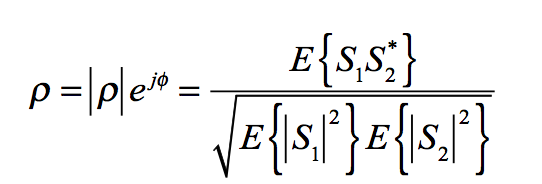
where E{} represents the mathematical expectation and * indicates the complex conjugate. In general, the terms from the complex correlation are refered as:
|ρ| : coherence
φ : interferometric phase
In case of SAR interferometry, the complex correlation coefficient is determined by different physical phenomena in such a way that its final value may be decomposed as a set of multiplicative factors [+]
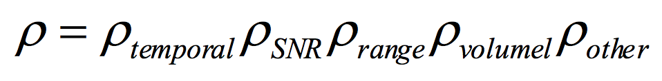
ρtemporal: defined as the ratio of temporarily stable scattering contributions to the total scattering intensity transferred to the SAR image. For repeat-pass systems, the temporal coherence accounts for the loss of coherence caused by scatterer’s changes that may occur between the two SAR acquisitions. Represents the most important decorrelation term in the frame of this study.
ρSNR: decorrelation induced by the thermal additive noises in both SAR images.
ρrange: known also as baseline or geometric decorrelation, appears as a consequence of the spatial separation between the positions of the satellite in the two acquisitions.
ρvolume: decorrelation induced by the presence of scatterers at different positions along the vertical direction. It may be employed to differentiate between short and tall vegetation covers, for instance, depending on the availability of longer baseline InSAR pairs.
ρother: any other decorrelation effect due for instance to data processing, orbital errors, etc.
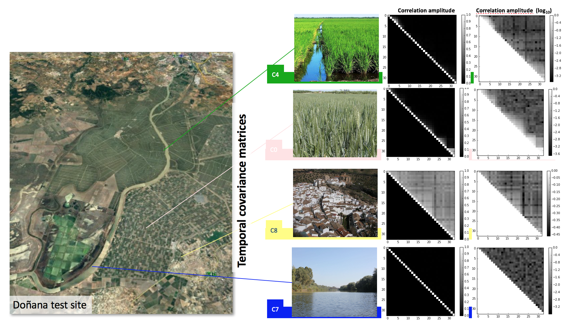
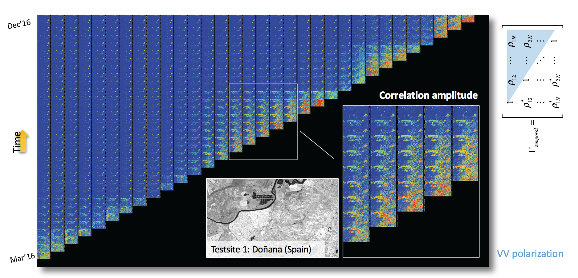
The multi-temporal covariance matrix
Given a temporal series of N SAR images S1, S2, …, SN, it is possible to define the Hermitian temporal Covariance matrix of a complete interferometric stack [+]
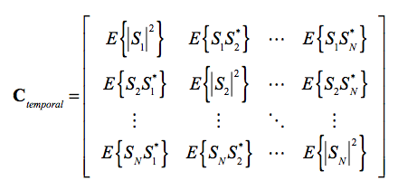
this matrix contains two types of information:
Radiometric information, contained in the main diagonal,
Interferometric information, contained in the off-diagonal terms
These off-diagonal terms contain in essence the coherence information of two SAR images.
The covariance matrix needs to be estimated from data, that is, speckle noise must be filtered out. Through the normalization of this matrix we can access to the multi-temporal coherence matrix[+]
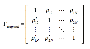
When considering the 6-day or 12-day coherence time series, we are basically considering the first upper diagonal. Nevertheless, both could be analysed at the same time by considering the 6-day time series of SAR images and then to consider the first and second upper diagonals. Moreover, it is also interesting to consider coherence time series formed with one master image, which in this case would correspond to single row or a single column. As observed, these coherence time series correspond to a subset of the multi-temporal information contained in the temporal covariance matrix, so these subsets may be insensitive to certain properties of the scatterer under observation.
Statistical considerations
In addition to the previous considerations, it is important to take into account the statistical description of the information contained in the covariance matrix as it determines the statistical properties of the estimated coherence values, but also how to consider the temporal information for classification purposes when considering multi-temporal information. Under the Gaussian scattering assumption, it is completely characterized by the complex zero-mean Wishart distribution and indeed, the covariance matrix itself characterizes completely the complete dataset of SAR images S1, S2,…, SN, that is, no additional data are necessary to characterize the data. On the other hand, a reduced subset of the elements, would be insufficient. For instance, the statistical approach has been widely explored in SAR Polarimetry for classification purposes through the so-called Wishart classifiers. These approaches are easily extendable to multi-temporal acquisitions.
Examples